PicoScope 7 Automotive
Available for Windows, Mac, and Linux, the next evolution of our diagnostic scope software is now available.
Automotive guided tests
Library of examples on how to perform tests when using PicoScope.

Training
Our collection of training videos, articles, guides and information on training courses.

Waveform library
The Waveform Library is a global database of waveforms uploaded by PicoScope users.

Case studies
Real-life case studies show how the professionals use PicoScope to diagnose vehicle faults.

A to Z of PicoScope
Detailed description of various PicoScope software and hardware features.

Videos
Training resources and demonstrations on PicoScope and the Automotive Diagnostics Kit.

Newsletter
Archive of our monthly Automotive Newsletters.

Documentation
Download manuals, brochures, posters, and training materials.

Reviews and awards
Accolades for the preferred diagnostic tool for service centers and vehicle manufacturers.

I finally got to revisit the Sherpa Van to determine why we experience a fluctuation in dwell angle of approximately 10° during the transition from idle to higher engine speeds.
The first thing to take into consideration was the potential movement of the distributor base plate due to the vacuum advance device or the centrifugal advance mechanism. Unfortunately, the vacuum advance diaphragm on the test vehicle was leaking, rendering the use of a vacuum pump near useless.
However, the application of a continual intake manifold vacuum was sufficient to overcome the diaphragm leak and rotate the distributor base plate.
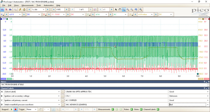
The waveform below displays the raw data before I applied maths, filtering and graphing:
The waveform below utilises the raw data we captured to visualise and graph the “real-time” effects of the distributor vacuum advance mechanism with relation to engine speed, ignition timing and dwell angle.
You can read more about graphing and filtering in the following forum post.
I used a WPS500X pressure transducer (on Channel D) in line with the distributor vacuum hose in order to plot the intake manifold pressure acting on the vacuum diaphragm. The engine was idling and we released the vacuum to the atmosphere by momentarily removing the vacuum hose from the diaphragm.
The effects of the vacuum advance (even with a leaking diaphragm) are dramatic for sure.
We used an optical pick-up on Channel A, aimed at the crankshaft pulley. This was generating one pulse per revolution, allowing for an accurate representation of engine speed. Note the drop in the engine speed when the vacuum was released from the diaphragm, given the ignition timing retards. (The optical pick up also proved invaluable during the following ABS case study.
Channel B shows the frequency of the peak firing voltages, or to put this another way, the ignition timing. Note how the ignition timing graph mirrors the engine speed graph.
You can find more information ignition timing graphing in the section “How did we calculate ignition timing?” further down in this piece.
The dwell angle on Channel C remains fixed throughout this whole event leading us to conclude that the vacuum advancement of the distributor base plate is not influencing the dwell angle.
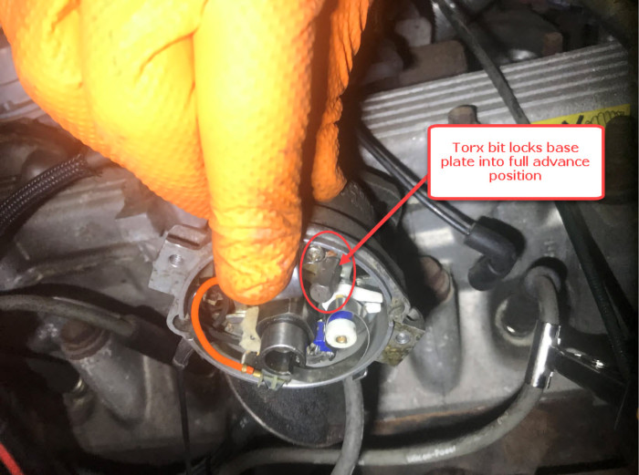
The next step was to determine if the centrifugal advance mechanism was influencing the dwell angle during the transition from idle to WOT. To do this, we locked the distributor base plate in the advance position, using a Tx20 Torx bit, and proceeded to run the engine from idle to WOT.
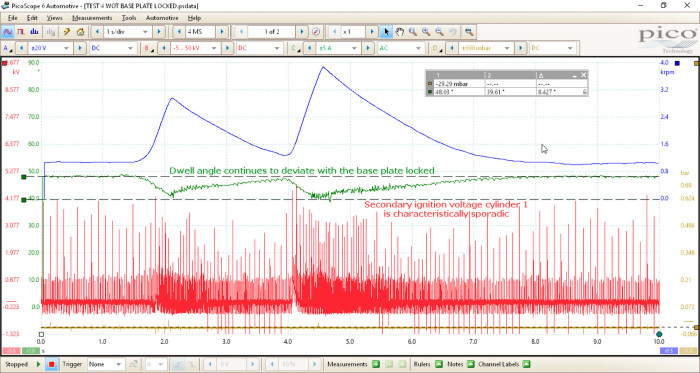
The screenshot below shows the engine running from idle to WOT and returning to idle with the distributor base plate locked in the fully advanced position.
This information makes us conclude that the deviation in the dwell angle is not linked to the operation of the vacuum advance device or the centrifugal advance mechanism. Therefore, the deviation must be a characteristic behaviour of the distributer assembly!
Previously I mentioned, “What I do know is the vehicle performs fine with no running or timing issues and mechanical inspection for lateral movement of the disturber shaft confirms no significant wear”.
Whilst the vehicle does run fine, “no significant wear” was not truly accurate under closer inspection.
The above video highlights significant lateral movement to alter the contact breaker gap from 15 thou (0.381 mm) to 24 thou (0.6096 mm).
Notice in the video below how the “floating” design of the base plate lends itself to the characteristic movement which alters the contact breaker gap
So I guess the question here is: “What does a good one look like?”
Once again, thanks to Kevin Ives, who pulled a brand new Lucas 59D4 distributor destined for a British Leyland A-series engine out of the bag (I kid you not).
In the video below, this brand new Lucas unit (complete with points and condenser) exhibits similar lateral movement of the distributor shaft, sufficient to alter the contact breaker gap from 16 thou (0.4064 mm) to 22 thou (0.5588 mm).
To conclude on dwell angle (and thank you for reading), the deviation we capture with PicoScope is a true event based on the design of the distributor and the dynamics that occur during the transition from idle to WOT. What we have highlighted, therefore, is typical behaviour and not a faulty or excessively worn distributor shaft bearing/bush, demonstrating one of the many reasons these ignition systems are no longer viable for today’s vehicles.
Next: With reference to Channel B capturing the secondary ignition event of cylinder 1, I want to clarify a number of questions that might be raised.
Using Deep Measure (read more in this forum post) we can locate each and every secondary ignition event for cylinder 1 while also revealing the time span between each event.
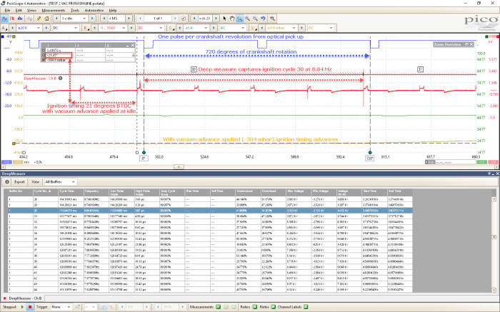
With the engine at idle speed, the time span between each firing event in cylinder 1 should remain near equal. However, when we apply vacuum advance, the time span will reduce. This resulted in an increase in frequency and advancement of the ignition timing. We can qualify this advanced timing using the rotation rulers to accurately measure the peak firing voltage in relation to the TDC marker (reflective tape) placed on the crankshaft pulley.
Ignition timing with -304 mbar of vacuum applied to the distributer
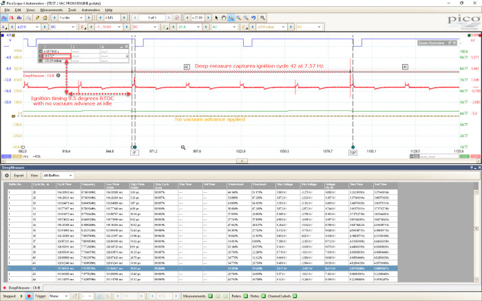
Ignition timing with NO vacuum applied to the distributor
How to graph ignition timing?
Realistically, we graph the change in the time between each firing event for cylinder 1. If the time between ignition events decreases, the frequency, therefore, increases and so we can conclude that there is an advancement in ignition timing.
Trying to graph secondary ignition voltages is challenging once we get above idle speed. Typically, secondary ignition waveforms are well defined at idle speed which helps both the math channel and Deep Measure. This is because to calculate frequency, you need a clear and well-defined crossing point.
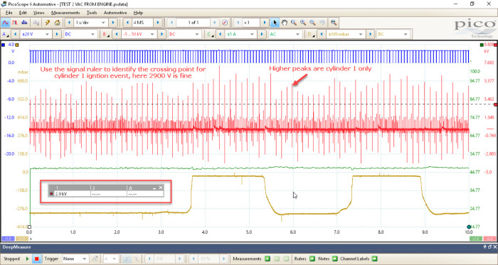
If we are to graph the peak firing-voltage events, we cannot use zero volts as our crossing point. This is due to the activity about zero volts from neighbouring cylinders and EMI (Electromagnetic Interference).
To overcome this hurdle, we can raise the crossing point of our signal to the chosen level above (2900 V) as only the peak firing voltages for cylinder 1will reach this threshold.
Amending the crossing point of a math channel
To raise the crossing point for channel B, use the math formula freq(B-2900). This goes for any math channel where zero is not the desired crossing point in which to determine the frequency of a signal. (Choose a crossing point relevant to your signal.)
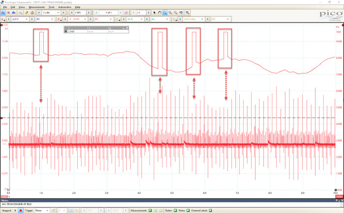
I mentioned how secondary ignition is challenging to graph, given that PicoScope can detect the slightest deviation or glitch in frequency. The results of such events can be seen below in the form of four peaks that deviate from the trend line.
Here, the math channel has captured a momentary increase in frequency in the ignition voltage, resulting in a deviation from the trend line. Bear in mind that this is at idle speed where ignition events are well defined.