PicoScope 7 Automotive
Available for Windows, Mac, and Linux, the next evolution of our diagnostic scope software is now available.
Automotive guided tests
Library of examples on how to perform tests when using PicoScope.

Training
Our collection of training videos, articles, guides and information on training courses.

Waveform library
The Waveform Library is a global database of waveforms uploaded by PicoScope users.

Case studies
Real-life case studies show how the professionals use PicoScope to diagnose vehicle faults.

A to Z of PicoScope
Detailed description of various PicoScope software and hardware features.

Videos
Training resources and demonstrations on PicoScope and the Automotive Diagnostics Kit.

Newsletter
Archive of our monthly Automotive Newsletters.

Documentation
Download manuals, brochures, posters, and training materials.

Reviews and awards
Accolades for the preferred diagnostic tool for service centers and vehicle manufacturers.

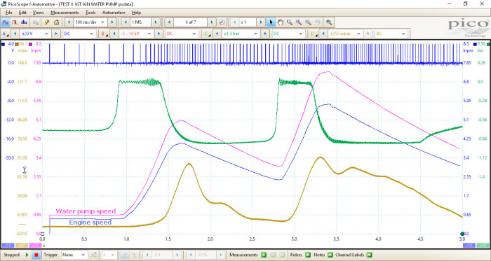
There are times when I could kick myself for not obtaining the crank sensor signal during a typical engine capture. While we may not be looking for a crank sensor related fault, it can help us graph the engine speed (https://www.picoauto.com/support/topic11511.html) during waveform analysis to determine if the engine/vehicle was accelerating, decelerating, etc.
We can, however, use other inputs to determine rpm and here is a typical example using an ignition trigger signal (IGT) from the number 1 Coil-On-Plug unit:
Below we have the WPS500X pressure transducer connected to the coolant expansion bottle in order to detect a change in pressure attributed to water pump impellor activity (confirming that the water pump impeller is actually rotating).

While the capture above appears cluttered, there are a number of software features in PicoScope that can be used to improve the view of the data we require.
1. Right click on the screen and hide Channel B (Ignition coil secondary voltage) as it is not required.
2. Close the Notes and Channel Labels to increase the size of your scope grid.
3. Click on the input ranges (V, Bar, etc.) and slide each waveform to a chosen position.
4. Use the Channel Option button to apply a “Lowpass” filter to noisy channels. (Channel A below has an 8 kHz lowpass filter applied.)

Now for the maths:
To obtain engine rpm from the IGT signal (Channel A) we need to know the number of cylinder 1 IGT events per engine revolution. As the number 1 IGT signal is present once every 2 rotations of the crankshaft we represent this as:
1 (IGT event) / 2 (Engine revolutions) = 0.5
We now need to convert “cycles per second” (Hz) to “cycles per minute” (RPM). One formula to remember here is: Frequency (Hz) x 60 = RPM, and likewise: RPM / 60 = Frequency (Hz).
So how does all this fit together in a math channel?
The formula required to obtain engine rpm from channel A is 60/0.5*freq(A) and can be seen below as applied in the math channel equation box in PicoScope 6.

Here we have graphed engine speed from 678 rpm through to a maximum of 5808 rpm.

Now that we have engine speed, if we know the relationship between the crankshaft and water pump pulleys we can obtain the water pump speed.
Example:
Crankshaft pulley: 175 mm
Water pump pulley: 145 mm
Using the formula “Driven / Driver”: 145 mm/175 mm = 0.83:1
0.83 rotations of the crankshaft to 1 rotation of the water pump
Engine at 1000 rpm / 0.83 = Water pump 1204 rpm
We can now create another math channel in order to graph the water pump speed. The formula is exactly the same as engine speed but now we include the water pump speed ratio: 60/0.5/0.83*freq(A)
I have included the .psdata file with the relevant math channels. Remember to use a lowpass filter on Channel A to 8 kHz. To view Channel B, right-click on the screen and select Channel B.
TEST 8 IGT IGN WATER PUMP.psdata
Food for thought here: an injector signal could also be used to graph rpm but remember that during overrun the injector signal will be cut and so there will be no data for the math channel calculation.
Also, with direct injection vehicles, we have the added complexities of variable injection strategies too, either during the induction or compression events and often during the same waveform time span.