PicoScope 7 Automotive
Available for Windows, Mac, and Linux, the next evolution of our diagnostic scope software is now available.
Automotive guided tests
Library of examples on how to perform tests when using PicoScope.

Training
Our collection of training videos, articles, guides and information on training courses.

Waveform library
The Waveform Library is a global database of waveforms uploaded by PicoScope users.

Case studies
Real-life case studies show how the professionals use PicoScope to diagnose vehicle faults.

A to Z of PicoScope
Detailed description of various PicoScope software and hardware features.

Videos
Training resources and demonstrations on PicoScope and the Automotive Diagnostics Kit.

Newsletter
Archive of our monthly Automotive Newsletters.

Documentation
Download manuals, brochures, posters, and training materials.

Reviews and awards
Accolades for the preferred diagnostic tool for service centers and vehicle manufacturers.

Working at Pico, I have the opportunity to look closer at some of the latest sensor technology that is out there on modern vehicles. While this particular sensor has been out there for a while now, SENT is cropping up in more and more vehicles.
The help desk, the Automotive Forum, and our FaceBook group have all seen an increase in questions and discussions around the best way to work with these sensors. This has prompted me to look into how PicoScope can be used to get as much information as possible from these sensors.
I’m not going to spend too much time on what SENT is. There are some great trainers out there that will do a much better job at describing how this protocol works. But let me give a brief insight into this network.
SENT stands for Single Edge Nibble Transmission and follows the J2716 standard. It is low-cost and uni-directional (one direction only), which means that the sensor can only send data out. What makes SENT different from other sensors is that multiple pieces of data can be 'sent' over one wire. One sensor can, for example, send both pressure and temperature measurements using a single wire. This makes it low cost and reduces the need for cabling, something manufacturers are always looking to do. This means you may well see a MAF sensor with just three wires which, when measuring, means you will have a 5V supply, a ground, and a data wire.
As I mentioned above, SENT can transmit more than one piece of data and it does this by creating a SLOW message from 'nibbles' taken out of the FAST messages. To build up a slow message, it takes multiple fast messages. The important note here is that both of these messages can be decoded in PicoScope by using the serial decoder.
So, what does a SENT data packet look like then?

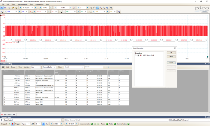
This capture is from a .psdata file that a member of the forum kindly uploaded. You can see the full forum post here: https://www.picoauto.com/support/topic21901.html.
You can see that it is quite easy to mistake it for a PWM signal given it is 0 – 5V with a seemingly varying change in duty cycle. You may also notice throughout this article that there appear to be inverted signals. This isn't deliberate. It is just another characteristic of the SENT protocol where the polarity of the signal can change but the data remains the same.
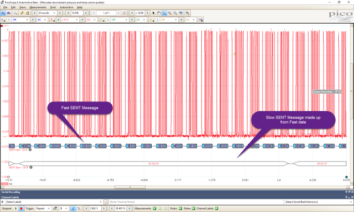
I will cover how to set each decoder up and add it to the signal, but just so we can all see how the SLOW signal is made up, I've already added the decoder to it. From this, we can see that there are several FAST packets of data required to make up the one SLOW message. This is important to note, as the SLOW message contains extremely useful information related to the sensor. Please note, however, that it is necessary to take a long enough capture to ensure you have all the data. I will post the best settings in due course.
If we continue to use the data above it is most practical to start with the SLOW decoder first.

Click Tools > Serial Decoding > Create> SENT Slow.
The reason I recommend you start with the slow message first, is that quite often you can find information about the sensor in this data, which is needed in order to set the fast decoder. The fast decoder provides you with several options as to how you would like the decoder to work based on the sensor type you are measuring.
To complete the decoder, the software will automatically set some parameters for the thresholds based on the channel selected. You will notice that this signal isn't 'clean' and that it has some interference. You can 'clean' the signal with the LowPass filter in the channel options. I've found that 300 kHz works well.
The other options are to amend the settings yourself, in which case, you will need to inform the decoder what voltage threshold to decode with as well as any hysteresis you would like to include. The following settings where done after the LowPass filter had been activated, but settings you can use would be 3 V with minimal hysteresis.
Once you are finished, click OK and make sure that the decoder is ticked before you click OK once more. A table will form at the bottom of the waveform some human-readable data. Unfortunately, we are still missing some additional sensor information. If we had a little more time on the screen we could get additional information on the sensor which in turn means that we can create a SENT Fast decoder more accurately.
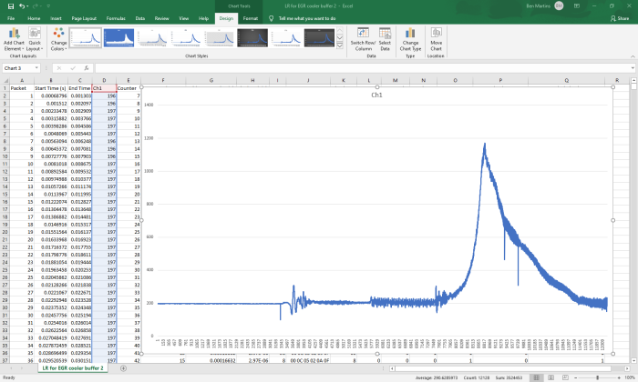
We could have continued with this capture and taken a guess at the type of sensor we had, but we had longer captures to decode with the additional information. I applied the slow decoder (following the previously mentioned process) to the following capture. For clarity, the sensor is a pressure sensor used in an EGR cooler. The capture was taken while the engine was started and through a snap WOT test.

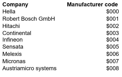
The more data packets present, the more chance we get to find some of the additional information transmitted in the SLOW signal. Packet 8 at this point is the one we are interested in. As you can see, it gives us the information relating to the sensor type. This is important when it comes to setting up the FAST decoder. We can see that we have a Pressure/Secure sensor. The additional data can be equally as important though, especially the Manufacturer code. The message ID refers to a list that can be used to determine who makes the sensor.
It is available with a quick search on the internet, but for reference, the ones that I've found so far are listed below –
Let's head back to PicoScope. In the serial decode tool, we select SENT FAST from the list.
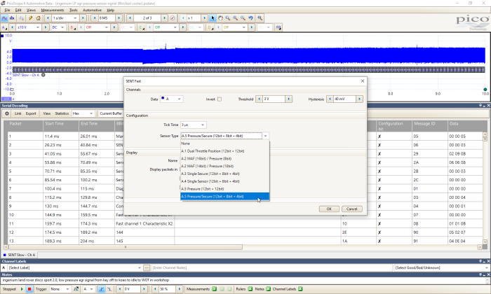
You will see that knowing the sensor type is important to us as we can select the specific sensor from the list. We know from earlier that it is a Pressure/Secure sensor. Again, I'm not going to go into too much detail here as it's not the purpose of the article but the format of the data field changes depending on the sensor type. PicoScope will allow you to pick out the type of format you want from the standard J2716 list.

Now we have both the Slow data and the Fast data in the decode table. To flick between the two, click on the tabs for each table at the bottom of the screen where the labels for the SENT Slow and SENT Fast are visible.
To better understand what the sensor is doing, the next step is to use the export function in PicoScope. In the decode table, make sure that you have the SENT Fast tab open and the decode operating on the current buffer only and click Export. You will then be asked to save the file in an easy to find location.
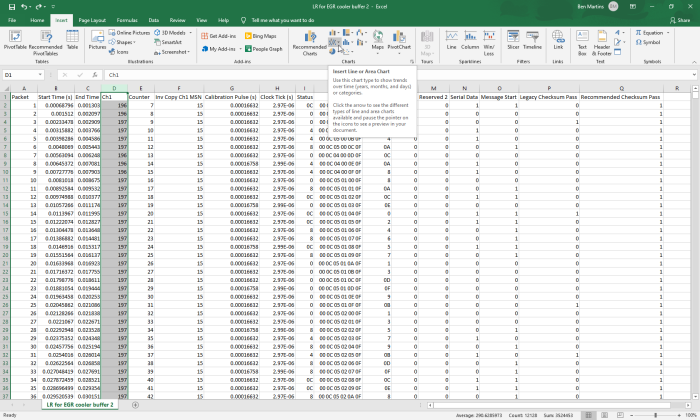
Locate the saved file and open it in Excel. You will now be presented with the decode table from PicoScope but with the ability to further manipulate the data. Steve has several posts on the forum where he has used Excel to pull further information from captured data. You can read more from Steve here.

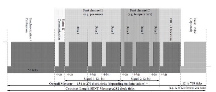
This can look quite overwhelming, but we are going to do something very simple to visualise what the sensor is doing, in a way we are familiar with. The data packet for the SENT message is split depending on the type of sensor, and they are labelled as Channel 1 and Channel 2. Below is an example which hopefully explains this in more detail.
When you apply the SENT Fast serial decoder in PicoScope, you are telling the software how you want the data to be split up. In the image above, this would be a typical even split for the data field so 12 bits for Channel 1 and 12 bits for Channel 2. We know that the sensor we are looking at in Pico is a Pressure/Secure sensor. When we look through the J2716 standard, the Pressure data is present on Channel 1. When returning to the Excel sheet, we can visualize the data by creating a chart. Select the Channel 1 column, column D

With the data selected, click Insert and locate the Line Chart option.
Now we have a graphed image of the data acquired from the SENT sensor. It may look a little basic, but we can zoom in on the graph by amending the data in the graph. I admit this is a little clunky, but it's better than nothing!
Selecting the data source and amending the data range will allow us to focus the graph on an area of data we would like to view more closely. In the graph below, I chose to view the data between D5625 and D12140.


In the graph below, I have amended the data range to between D5625 and D6625. I think we can agree that what we are looking at resembles an exhaust pulsation waveform.

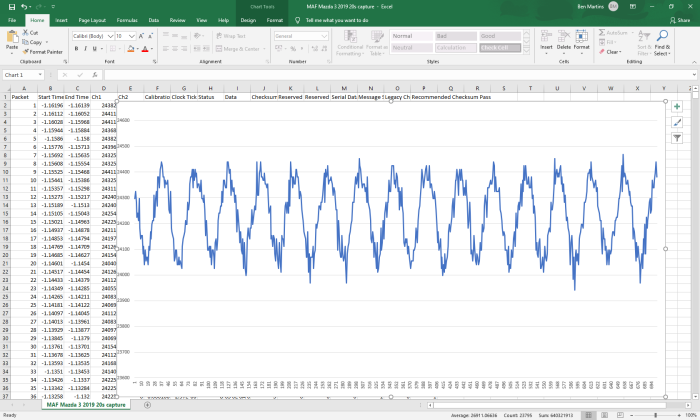
Below is the same process applied to a MAF sensor using a SENT sensor to send out airflow and temperature. I captured the data with PicoScope, decoded it and exported it. Then I created a chart from the data on Channel 1. I also carried out a similar test with the engine idling before moving to a WOT snap test.

Here is the zoomed-in version that we achieved by amending the range.
There is, however, one slight problem that I've run into so far. I can't correctly take the value decoded for channel 1 or 2 and translate this into a unit of measurement we can relate to. The way the data is translated from the sensor is from the characteristics present in the SENT slow message. Kim Anderson has done some amazing research into this already and has kindly updated the forum post that inspired this article.
I have yet to successfully use these to determine the true measured value. That being said, I feel that this is an extremely useful way of visualizing a sensor in a way we couldn't before. I guess you could graph the data from a serial scan tool. I would, however, be worried that the refresh of PID data will miss something, which could be vital for intermittent faults.
For both the exhaust sensor and MAF sensor I've found it best to take a long capture, between 1s/div and 2s/div, and keep the sample rate high (aim for 10MS). This will hopefully ensure that the samples can be decoded correctly. I have seen that I get the yellow warning triangle for 'Sample rate may be too low.' I've not had any issues with the decoding so far. You can make sure you avoid any loss of data, by adding a single trigger but you have to be ready to perform the snap test. We will continue to work on trigger functionality as it’s one thing I've found tricky when capturing. Other options would be to use another channel for the accelerator pedal position or the brake switch. Once you're all set up, a quick touch of the pedal will trigger the scope ready to capture the data for decoding.
I hope this helps and please feedback with any suggestions and if I can get the units working, I will update.
This article was inspired by a case study on a forum thread that has also been added to by other users. You can find the forum thread here.