Calculating theoretical MAF 

With reference to the following case study.

I thought it would be good to revisit the maths and modify the technique to calculate the theoretical MAF. Thanks to Andy Crook at GotBoost and the comments left at the end of the case study they are always appreciated.

Like with all measurements, accuracy is paramount and there will always be variables where maths is applied to raw data. Hopefully, the information below will help minimise inaccuracies attributed to how maths and filters are applied.

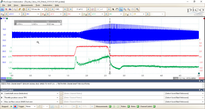
Here we have a 1.8-litre, 4-cylinder, normally aspirated Toyota Celica (engine code 2ZZ-GE).
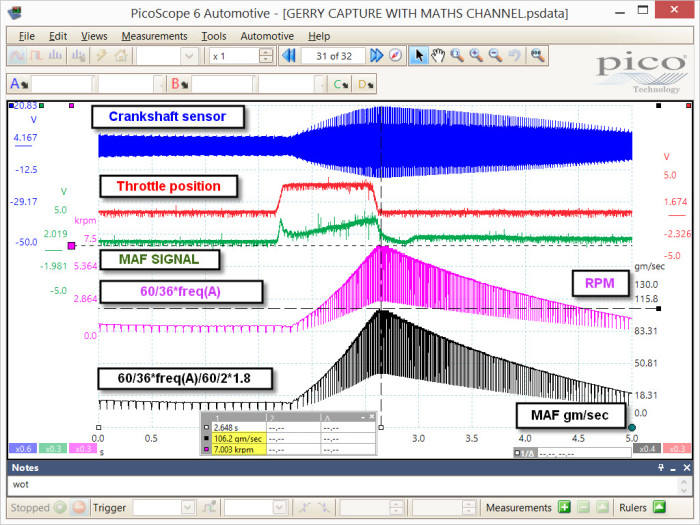
Our capture focuses on the relationship between the crankshaft sensor, throttle position and MAF, from idle to WOT.

To accurately determine the maximum engine speed during the WOT event, I have zoomed in at the point of peak amplitude to measure one engine revolution with the time rulers. 
Note: with an inductive style crankshaft sensor the amplitude increases in proportion to engine speed.

The math channel Crank(A, 36) is also included to graph the engine speed (topic11511.html).

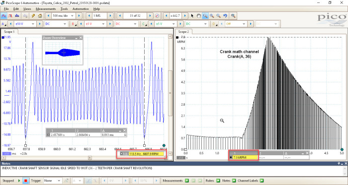
As we can see above, there is a discrepancy between the measured value at higher engine speeds when using the accurate time ruler method on the left (6807 rpm) and the crank math channel on the right (7000 rpm). 

We also have the presence of those “nuisance spikes”, where the software detects the instantaneous dramatic increase in signal frequency, immediately after the missing teeth. 
This has been documented and will be resolved given that the crank math channel should not draw data where the missing teeth pass the crankshaft sensor; instead, it should seamlessly display data as the remaining teeth continue "en route".

We can tackle the crank math channel concern (nuisance spikes) by using the filtering function of math channels. 

post86291.html#p86291

https://www.picoauto.com/library/training/filtering

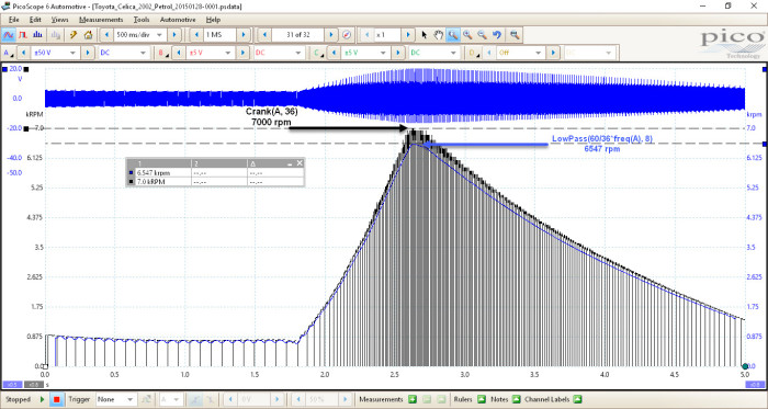
The crank/rpm math channel would (as usual) utilise “frequency” and be re-written as LowPass(60/36*freq(A),8) to incorporate an aggressive lowpass filter of 8 Hz.

Above, we can clearly graph an overview of engine speed without the intrusion of nuisance spikes. 

Below, we can compare the crank math channel with the filtered rpm math channel.

The LowPass(A, 8 ) section of our equation applies an 8 Hz lowpass filter to the rpm math channel, which has the benefit of removing the nuisance spikes (for ease of viewing) but at the expense of peak accuracy. 

Our initial rpm measurement (using the time rulers), confirms our peak rpm to be 6807 rpm, whereby the blue lowpass math channel above indicates 6547 rpm, which is 260 rpm adrift. 

If we are just after an indication of rpm activity this rpm math channel is fine, but if we want to calculate theoretical airflow we need an accurate peak rpm value where our math channel matches our measured value obtained using the time rulers.

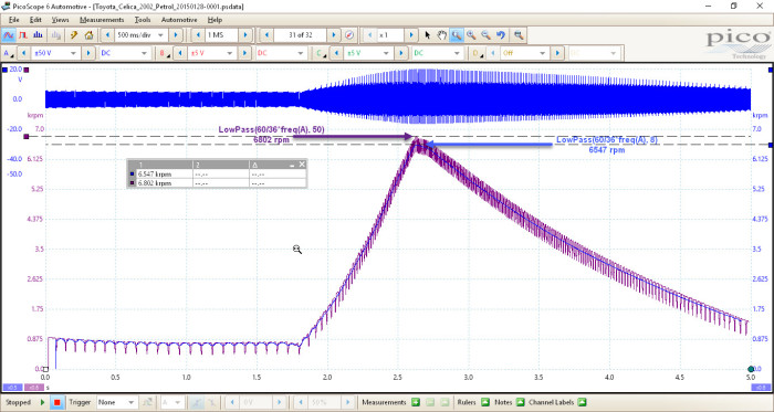
We can achieve the correct peak rpm by amending the amount of lowpass filtering we include in the math channel.

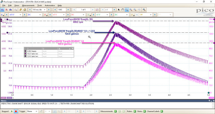
Below, we have LowPass(60/36*freq(A), 50) where our peak rpm is now accurate (6802 rpm), with minimal intrusion from those nuisance spikes, thanks to our 50 Hz lowpass filter included in the math channel. Depending on the type of crankshaft sensor in your application, choosing the correct lowpass filter setting in the math channel will be trial and error.

Now we have an accurate math channel indicating the correct peak rpm, we can move onto our theoretical MAF calculation.

Calculating theoretical MAF values:
MAF = (RPM X ENG CAPACITY in LITRES) / (60 X 2 INTAKE STROKES PER REVOLUTION)
While there are several routes to arrive at the same MAF value, I will break it down as follows:
Using the process below, we can estimate MAF for a normally aspirated engine (assuming a WOT).

Example 
Our normally aspirated Celica uses a 1.8 litre, 4-cylinder, 4-stroke engine.
Assume now this engine is running at 3000 rpm (WOT) the airflow consumed could be calculated as follows: 

3000 RPM / 60 = 50 rev per second (Hz)
For a single revolution of our 4-cylinder engine, we have 2 x intake strokes.
Therefore, 50 rev per second x 2 = 100 intake strokes per second.
Each intake stroke = 1.8 litre / 4-cylinder = 0.45 litre (450 cc) per cylinder.
100 intake strokes X 0.45 litre = 45 litres per second.Note: Air mass is approximately 1 gram per litre at sea level (pressure and temperature-dependent).
Therefore, 45 litres per second is approximately 45 grams per second (45 gm/sec).

With that said, aerodynamic calculations are based upon air mass at sea level at 15 degrees centigrade being approx. 1.223kg/m3 or 1.223g/l.

Here then, we multiply our 45 litres per second by 1.223 to obtain 55.035 gm/sec.

Be aware that all the above assumes the volumetric efficiency (VE) of our engine to be 100 %, where in reality, we can pray for 90% at peak torque (a true reality check is more like 86 to 88 %).

The math channel would be written as follows:
LowPass(60/36*freq(A),50)/60/2*1.8 for air mass at 1 gram per litre

For air mass at 1.223 g/l the math channel would be written as follows:
LowPass(60/36*freq(A),50)/60/2*1.8 x 1.223

Above, we now graph the theoretical MAF across the entire rev range using both values for air mass (assuming 100 % VE). I guess the question now is which values are used for air mass by the vehicle manufacturer (1 gm/l or 1.223 gm/l) and what values are displayed on their data lists? Food for thought for sure.

VE calculations. 
Calculating VE is challenging regardless of ability or formulas as the complexity surrounding manifold configurations, throttle positions, valve duration/lift and aerodynamics do not lend themselves to a simple formula.
However, as a baseline calculation of VE, we can use airflow figures.

We can never assume that an engine has a 100% VE, but if we calculate airflow assuming our engine has 100% VE using the airflow formula, then using a scan tool (gm/sec), we can obtain an approximation of the actual VE using the difference obtained from the scan tool compared to the value obtained via the scope formula. (This is assuming that the air mass meter is performing correctly, with no air leakage post-MAF meter and an engine with no performance issues.)

In the aforementioned case study, the math channel used below, 60/36*freq(A) indicates an rpm of 7004 rpm with theoretical MAF of 106.2 gm/sec (assuming 100% VE and air mass at 1 gm/litre). 

Interestingly enough, the throttle is closed at the peak rpm and MAF measurement points of the math channels! This may be due to a combination of how math channels are applied/calculated and how engine speed does not immediately fall at the instant of the closed throttle. Remember we are calculating peak MAF based on calculated rpm.

The Scan Tool reveals MAF to be 111.85 gm/sec at a similar rpm of 7021 rpm

If we now do the maths on these figures, the scope has calculated MAF to be 106.2 gm/sec whereas the Scan Tool reports MAF to be 111.85 gm/sec at a similar rpm.
111.85 / 106.2 = 1.05 x 100 = 105 % Volumetric Efficient (VE)… It’s a miracle!

While this engine utilises VVT-iL “Variable Valve Timing and Lift” (valve lift increases at high rpm), it is certainly not over 100 % volumetrically efficient and does not suffer from external air leakage (post-MAF meter) to warrant such airflow.

If we now use MAF at 1.223 gm/litre its starts to look more applicable 
The scope has calculated MAF to be 106.2 gm/sec x 1.223 = 129.88 gm/sec
The Scan Tool reports MAF to be 111.85 gm/sec 
111.85 / 129.88 = 0.86 x 100 = 86.11 % VE
 We can, therefore, conclude that the manufacturer in this instance is displaying MAF values using 1.223 gm/litre (based on our calculations), with the vehicle performing correctly.
To summarise: If we know the engine speed, the number of cylinders and the engine capacity we can calculate the theoretical airflow.

One final amendment to your math channel could include an average VE value of 88%.
If we had used the math formula LowPass(60/36*freq(A),50)/60/2*1.8*1.223*0.88 within the case study, we arrive at a typical MAF value assuming 88% VE rather than 100%: 129.88 gm/sec * 0.88 = 114.29 gm/sec (Scan Tool = 111.85 gm/sec).
 I am not sure if this helps as it is useful to calculate VE (post-capture) based on the theoretical MAF at 100% VE against the reported MAF from the scan tool, but it remains an option if required.

The psdata file can be found below. You will need to download the latest PicoScope software to view the file.

Toyota Celica MAF.psdata

I hope this helps and reveals the many challenges we face using these techniques.

Case study scan data