Maths is cool - part 16
by Steve Smith

Following a recent inquiry via the support desk surrounding the operation and diagnosis of an Electronically Commutated (EC) fuel pump, I thought it would be a great topic to share here.

The principle of EC is something we must learn to grasp, as it is the same technology that will be powering the vehicles of the future (hybrid/electric vehicles (EV)) via 3-phase motors.

To make a long story short, we have a 3.0-litre V6 gasoline Audi SQ5 with the engine code CWGD.

The fuel pump (G6) is failing to deliver adequate fuel pressure.

N.B. The fuel pump (G6) is integrated into the fuel sender assemblies, all in a single fuel delivery unit (GX1) immersed inside the fuel tank. The control of the fuel pump is via an external fuel pump control unit (J538) where the conversion from DC to 3-phase AC is implemented.

To quote Ben Martins: “Pressure is generated by the opposition to flow”. Bear in mind that our fuel pump is required to generate sufficient flow of fuel from the tank to the engine under all load conditions.

The image below reveals how we connected the PicoScope 4823 to simultaneously capture the 3-phase voltage and current to the offending fuel pump.

So why use such an elaborate control system for a fuel pump?

Performance, finite control, reliability and durability are the collective answers. Motors such as these are virtually wear-free, other than the support bearings. Due to the absence of motor brushes, there is no contact between moving motor parts. This eliminates, friction, drag and arcing. (These motors are referred to as BLDC = Brushless DC.)

For a typical wear pattern from a brush type motor, take a look at the images here and here.

Rather than me trying to explain how the EC motor functions, you could take a look at this superb animation.

As you can see, to make the rotor spin, we need to generate a rotating magnetic field about the stator that the rotor will “chase”. If we then attach the rotor to a pumping element, we can capitalize on the rotation and convert this motion into a physical pressure.

The same principle applies to any application, be that an EC motor connected to a transmission, road wheel or output shaft.

In the following screenshot, we have zoomed in to focus on the behavior of the voltage and current during the operation of the pump/motor. Notice how the voltage appears cut off at 0 V for channels A, B and C, yet the current is reversed during this period!

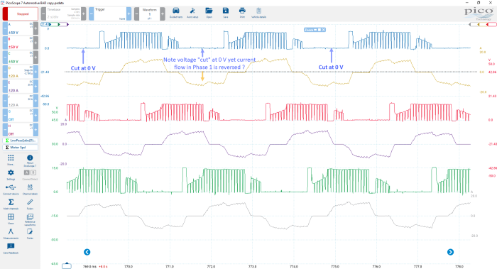
Our DC voltage captures do not tell the full story, as we are measuring with reference to chassis ground (which is correct). In reality, the voltage here is reversed in order to reverse the current flow we have captured in the phase windings on channels D, E and F.

Should you wish to capture the reversed voltage, a differential probe would be required to measure across the phases of interest. Especially for high-voltage applications, which also require the relevant training and certification for live working.

With all that said, by measuring “current flow” you can reveal the full story in a non-intrusive fashion and provide evidence of “work done”.

Measuring current reveals:

• Additional operational characteristics of the motor (within the waveform)

• The integrity of the magnetic field/coil windings

• The operation of the motor/pump

• The control circuit functionality

• Motor frequency/speed

• Motor load conditions

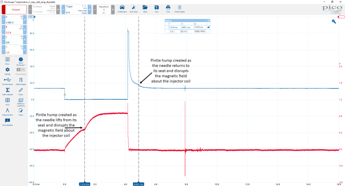
Let me digress for just a moment: The influence of magnetic fields on voltage and current are well documented. One of the best examples I have found is the disruption we capture when measuring current flow into a port injector. Below we capture the initial pintle movement (injector open) as it disrupts the magnetic field (and so current flow) about the coil windings and again in the induced voltage (back EMF) on the return to its seat (injector closed).

So how does this relate to our BLDC motor?

The waveform below indicates the momentary disruption during peak positive and negative current events where the rotor poles align with the stator poles at “peak north” and “peak south” respectively.

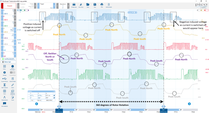
Even more interesting is the voltage on channel A in Image 4 and the grey rectangles placed about the start and near-end points of each positive phase. (All voltage phases have the same characteristic.) This is the induced voltage created within the phase winding when the current switches from on to off (back EMF) and it is used by the fuel pump controller to determine the position of the rotor. (How cool is that?) No need for an additional resolver or hall-effect position sensor in order to determine rotor position.

Knowing the position of the rotor is essential to determine the energizing sequence of the stator windings to create a rotating magnetic field (EC) for the rotor to chase.

Note: We cannot see the reversed induced voltage at the near endpoints of each voltage phase for the reasons mentioned above (See paragraph beneath image 2). With that said, we can see a gap where this negative induced voltage would appear shortly before the commencement of the missing negative voltage phase.

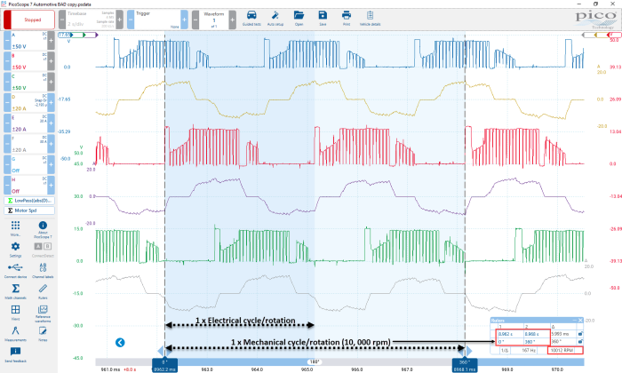
One further point, before we move onto the maths, note the number of electrical cycles/rotations in relation to one mechanical rotation of the rotor/pump.

The multiplication factor between electrical degrees of rotation (cycles) and mechanical degrees of rotation, requires knowledge of the number of poles about the rotor:

Multiplication factor = Number of rotor poles / 2

Therefore, our pump contains a 4-pole rotor (1 pair of north and 1 pair of south poles)

Number of rotor poles 4 / 2 = 2.

2 is the multiplication factor between electrical cycles and mechanical degrees of rotation for a 4-pole rotor.

In other words, for a 4-pole rotor, we require 2 electrical cycles for the rotor to complete one revolution

If you don’t know the rotor pole count you can use an optical pick-up sensor to capture one mechanical revolution of the motor assembly (where access permits) while simultaneously capturing current in one of the three phases.

Count the number of electrical cycles between the output events of the optical pick-up and multiply by 2 to find the pole count. The image below uses this technique to reveal a 30-pole rotor from a different style 3-phase motor.

Be aware that some rotors may not be linked directly to the mechanical output you are capturing with the optical pick-up due to reduction gears, etc. This would most certainly return an erroneous rotor pole count.

Let’s return to the faulty fuel pump. What can we diagnose from the original capture (Image 1)?

I’m using the following math channel LowPass((abs(D)+abs(E)+abs(F))*0.333,50) to determine the average current consumed by the fuel pump (incorporating all three current phases).

• LowPass smooths out the AC ripple and gives you a moving average.
• abs(D)+abs(E)+abs(F) * 0.333 gives the average of the three rectified phases (current).
• ,50 describes the level of low pass filtering applied (50 Hz).

 

To calculate the rotor/pump speed the math channel formula is 60*2*freq(D)/4 (60 x 2 x frequency of a current phase / rotor pole count).

• 60 converts Hz to RPM.
• Multiply by 2 because of the positive and negative events of the AC current waveform.
• Divide by 4 because our rotor has 4 poles.

Note: The rotor/pump speed depends on the frequency of the current and the rotor pole count.

• Increasing the frequency will increase the speed but reduce torque

• Increasing the rotor pole count will decrease speed but increase torque

Above we can see the fuel pump running at a fixed speed of 10,000 rpm and drawing an average current of 7.6 A.

Let’s now compare this to the waveform captured after the pump replacement:

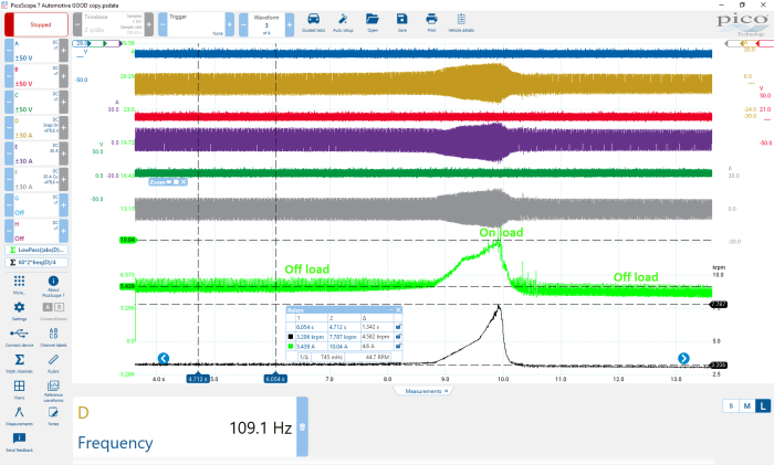
There is most certainly a difference. Look at the pump speed and current draw: up to 8 seconds, approximately 3200 rpm and 5.4 A (off-load). Also note how the frequency of the current (Channel D) between the time rulers has reduced to 109.1 Hz, resulting in a reduction in pump speed.

Now look at the pump speed and current when the pump is forced to deliver maximum pressure (on- load), approximately 7787 rpm and 10.4 A.

To summarize:

The new fuel pump pulls 5.4 A @ 3200 rpm to maintain sufficient fuel pressure during the off-load stage (less current and less speed for sufficient fuel pressure). The original pump pulled 7.6 A @ 10, 000 rpm for insufficient fuel pressure.

Most certainly, measuring the current reveals the “work done” and never is this more evident than during the pump “on-load” test we have captured in image 8.

So, what was wrong with the old fuel pump?

The simple answer is nothing! Remember that pressure is generated by an opposition to flow and the fuel pump activity captured in image 7 is most certainly creating flow at 10,000 rpm, but where is the flow going? Take a look at the fuel pressure regulator diaphragm that is integrated into the fuel delivery unit (GX1).

The diaphragm inside the fuel pressure regulator is torn, resulting in the majority of our fuel flow returning to the tank rather than along the fuel lines to the engine bay.

If you want more information on this style of fuel delivery system, try searching for the VAG Self Study Program SSP495.

Many thanks to our Audi colleagues overseas for their invaluable input in this case study.