PicoScope 7 Automotive
Available for Windows, Mac, and Linux, the next evolution of our diagnostic scope software is now available.
Automotive guided tests
Library of examples on how to perform tests when using PicoScope.

Training
Our collection of training videos, articles, guides and information on training courses.

Waveform library
The Waveform Library is a global database of waveforms uploaded by PicoScope users.

Case studies
Real-life case studies show how the professionals use PicoScope to diagnose vehicle faults.

A to Z of PicoScope
Detailed description of various PicoScope software and hardware features.

Videos
Training resources and demonstrations on PicoScope and the Automotive Diagnostics Kit.

Newsletter
Archive of our monthly Automotive Newsletters.

Documentation
Download manuals, brochures, posters, and training materials.

Reviews and awards
Accolades for the preferred diagnostic tool for service centers and vehicle manufacturers.

In this guest appearance, Ben Martins covers:
I have recently been carrying out some work using Pico Technology’s Engine and Hydraulics Kit and flow meters. These allow me to look at both the engine and the hydraulics side of a machine in order to determine faults with either or both sides of the system.
A common test to determine the hydraulic pump serviceability is something called a PQ test. This is where you push the pump to its maximum system pressure to ensure that it is capable of still producing the correct flow at certain pressures. When done at regular intervals, this test can be used to track the pump’s operation and catch any sign of significant wear or drop in performance before it is too late.
With Pico’s 300 Lpm and 600 Lpm flow meters, it is possible to carry out a PQ test and use the loading valve to ‘load’ the pump and record the data rather than file everything on paper. Additionally, once a stored file has been created, the setup is done for you and you only need to connect to the machine to run another test. Now, where does the maths come into it?
Something I find useful in hydraulics is comparing a theoretical flow rate to that of the actual and calculate the volumetric efficiency of the pump. Understanding how to set up your scope and what signals you need to capture will be based on the formulae we will be using. To begin with we need the theoretical flow rate, which is as follows:
Theoretical Flow (LPM = Pump Displacement (cc/rev) x Pump Speed (RPM) / 1000
If you’re using gallons per minute then the formula will read:
Theoretical Flow (GPM) = Pump Displacement (cu ins/rev) x Pump Speed (RPM) / 231
Being in the UK, I will be using the first formula as the pumps here are marked in cc/rev. For this exercise, the pump has a displacement of 51 cc/rev. We need to be mindful that this theoretical calculation is based on a pump being 100% efficient, which is not possible due to internal leakage. However, having both will allow us to calculate efficiency.
We also need to gain the pump speed. For most mobile hydraulic machinery, the pumps will be directly connected to the engine: engine speed = pump speed. This makes it easy to gain pump speed, as we can use the engine crankshaft position sensor or other signals to determine it. If the pump is driven externally from the engine, maybe from a belt or a gear, the speed can be acquired from an optical pick-up, or you can calculate the ratio between the crankshaft and the gear and factor this into the formula. For my example, the engine and pump are directly linked but we still need to convert the crankshaft position sensor output into RPM.
During this test, I will be fixing the engine speed to a set figure of 1500 RPM. This is a good operating speed for most machines but also acts as a constant when we carry out the test again in the future. Remember that all this information can be added to the notes section in PicoScope which will remain with the file. That way, if someone else has to carry out the test in your place they can follow the same test plan. In this case, we could opt to use the crank math channel, but as the RPM is fixed I’m not really that interested in the fluctuations of engine speed from a diagnostic point of view. For this reason, I will use a filtered frequency math channel as per the following forum topic. This will provide me with a much smoother line but will still show larger engine speed changes due to the loading and unloading of the pump.
The math behind this comes from the forum topic, but I have adjusted it slightly to account for the RPM on this machine. As we have a 37 tooth pick up ring on the crankshaft sensor, we need to add a scaling factor to ensure our RPM is correct. In this instance, I’ve used 1.616. The formula, therefore, reads as follows:
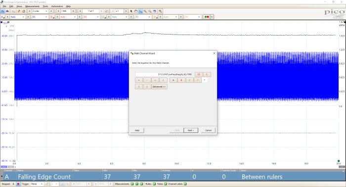
RPM = 1.616 x LowPass(freq(A),4)
To confirm your RPM, it is good practice to zoom in on your crank signal and use the time rulers to confirm the RPM.
1. Ruler overview with measured math channel
2. Math channel
3. Frequency and RPM measured between time rulers
From the above, I’m happy that there is minimal difference between the two and so the math channel can be saved and renamed for future use. To calculate our theoretical flow rate from here, we need to put the math channel we have created for RPM into the formula from earlier. This means creating a new math channel of the following:
Theoretical Flow (LPM) = Pump Displacement (cc/rev) x Pump Speed (RPM) / 1000
= Pump Displacement (cc/rev) x Pump Speed (RPM) / 1000
= 51 x (1.616 x LowPass(freq(A),4)) / 1000
Now we have engine speed and a theoretical flow rate based on our pump speed and pump displacement of 51cc/rev.
Now to the PQ test, which requires a connection into the hydraulic system to measure the flow and the pressure. Please ensure that you have the relevant training and correct PPE and that you prevent any potential contamination that could occur. This includes checking any hoses, fittings, and the WPS600C pressure transducer as well as the flow meter for cleanliness.
With the system installed, make sure you are aware of the working pressure of the machine. Begin to load the pump and remember to always keep observing the pressure. Pico’s flow meters do come with a safety burst disc which gives you some protection in the event of a pressure spike or if the loading valve is wound too far. Bear in mind that any burst disc will have to be replaced before you can carry out any further testing.
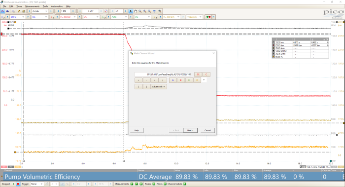
The below capture is from a machine with a working pressure of 260 bar.
1. Engine RPM math channel
2. Pump pressure
3. Measured flow
4. Theoretical flow
5. Unloading of the pump
6. Ruler overview
I want to focus on the first part of the capture, between the time rulers. You can see that the pump pressure is 255 bar. Due to the connection, we are not protected by the relief valve, which is why I have limited the pressure to below the working pressure. This ensures safety but also gives me a good indication of the pump’s output. The important measurement here is the flow rate because flow makes it go. By using the rulers, we can see that at 255.5 bar we have a flow rate of 70.25 LPM. Comparing this to our theoretical flow rate of 78.75 LPM we are losing about 8 LPM. Knowing that all pumps are never 100% efficient this could be down to the natural internal leakage I mentioned earlier. All we have to do to calculate the volumetric pump efficiency is to divide the actual flow rate by the theoretical and then multiply by 100 to get the percentage.
Pump Volumetric Efficiency (%) = (Actual Flow Rate / Theoretical Flow Rate) x 100
In the above capture this would read as follows:
Pump VE = (70.25 / 78.78) x 100
=0.89 x 100
=89%
We could leave it at that or we could include this in the capture using another math channel. Remember that you can add as many math channels as you like post-capture, as it leaves our original data unaffected. The resulting formula is, therefore:
(D/(((1.616*LowPass(freq(A),4))*51)/1000))*100
To make it a little easier to read, I have added an average measurement to the math channel between the two rulers indicating when the pump is being loaded.
I have attached the PSDATA file with the appropriate formulae. The power of math has the potential to reveal so much more and there are many more calculations we can do with hydraulic formulae which I hope to bring more of in the future.
PSDATA file: PQ Test with math.psdata