PicoScope 7 Automotive
Available for Windows, Mac, and Linux, the next evolution of our diagnostic scope software is now available.
Automotive guided tests
Library of examples on how to perform tests when using PicoScope.

Training
Our collection of training videos, articles, guides and information on training courses.

Waveform library
The Waveform Library is a global database of waveforms uploaded by PicoScope users.

Case studies
Real-life case studies show how the professionals use PicoScope to diagnose vehicle faults.

A to Z of PicoScope
Detailed description of various PicoScope software and hardware features.

Videos
Training resources and demonstrations on PicoScope and the Automotive Diagnostics Kit.

Newsletter
Archive of our monthly Automotive Newsletters.

Documentation
Download manuals, brochures, posters, and training materials.

Reviews and awards
Accolades for the preferred diagnostic tool for service centers and vehicle manufacturers.

| Vehicle details: | DAF CF |
| Symptom: | Cutting out |
| Author: | Ben Martins |
It seems that a lot of the faults I come across these days are communication-based and this vehicle is no different. Having a good understanding of how an automotive network is created is becoming more and more important, but fundamentally it is just about voltage. Don’t panic straight away, just because there are 30 fault codes all shouting communication issues. There are some simple and basic things we can do to determine what is going on, and with PicoScope, we can delve even deeper.
Talking to the customer is one of the most important tasks in any diagnostic job. They have all the information about the vehicle and may hold that key piece that was missed on the job card. The complaint this time is: the vehicle suddenly cut out and then wouldn’t restart. Using a little intuition may help in this situation so open-ended questions can lead to further information from the customer. Keep them talking. Ask them about the weather, how long they were driving, if this fault has happened before, if any other work has been carried out recently, any warning lights on the dash before the fault happened, the speed they were doing, what gear, and so on. As it turned out, the important bits of information I got from these questions was that the vehicle was fine from cold but after driving for some time it suddenly cut out. They were waiting some time for the recovery services who naturally attempted to restart the vehicle, and behold; it started again! However, setting off with the recovery services following, it wasn’t long before the engine cut out again. It would be wrong to assume anything at this stage, but I thought we could be looking at a temperature related fault.
Coming to look at the vehicle the next day meant that it had plenty of time to cool down and we were able to look at the vehicle in the same conditions as the driver did right before the fault occurred. Also, you should never overlook serial diagnostics if you have the opportunity to take a look. They can often point you in the right area but may not always have the answers. In this case, we had 12 active diagnostic trouble codes of which 11 are reporting CAN communication faults. To add further detail 4 of these were directly pointing to the Engine ECU. While not completely obvious at this time, it does help gives us some direction. With this in mind, I felt it was necessary to observe the CAN lines to the Engine ECU.
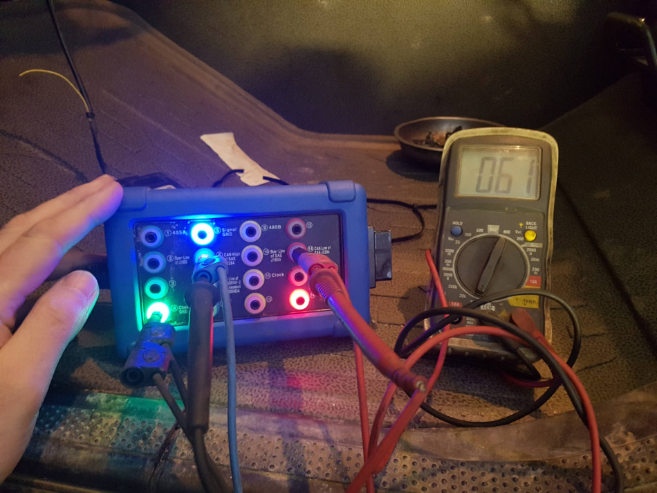
Verifying how the network is set up is a must at this point, as there are several networks on all vehicle types. This could mean that an ECU of interest might not be on the network you are connected to, so always double check a wiring diagram. For us, the ECU of interest was the Engine ECU and it happened to be involved in a number of networks including one that with the OBD port in it. This network was a typical setup, utilising two 120 Ω terminating resistors joining CAN H and CAN L together. These will normally be situated in an ECU at the end of the network, and so a simple resistance check on the CAN network can be carried out to verify its integrity. Here we could utilise the breakout box to easily gain access to the terminals, but we could also confirm the network was no longer active and shut down. It is good practise to only carry out a resistance check to a network when it is no longer active, and normally you would disconnect the battery to prevent the network from waking up. Disconnecting the battery on this vehicle was not practical due to some additional equipment fitted, so observing the breakout box LEDs for inactivity was the next best thing. We could also use the PicoScope to watch and wait for the network to shut down to be completely confident but as I said, best practise is to disconnect the battery.
With the network no longer active, a quick resistance check saw the magic 60 Ω we would expect to see from two 120 Ω resistors in parallel.
Next on the list was to try and catch the fault in action. For this, we utilised PicoScope’s ability to capture against time and hopefully catch the point when the fault occurs. We’ve done a lot on CAN lately and even put together a video for an overview of CAN diagnosis along with two guided test videos. In the diagnostic and decoding video, where we talk about how to set the scope up for analysing a CAN network, some typical faults, and how to decode the data.
We didn’t strictly follow the tests in this situation, as we aren’t dealing with a typical fault, although the first stages of verifying the integrity of the signal remain. We have a new guided test on how to test the CAN Bus physical layer:
Moving onto capturing the fault, we wanted to extend the time to allow for more data on the screen. I’ve used 2 ms/div which gives us more time in total but allows us to maintain enough detail to decode on.
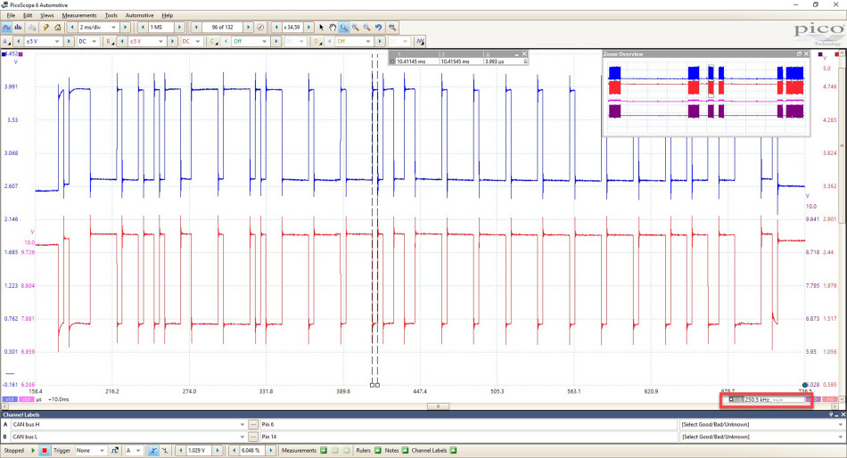
If you’ve followed any of our previous case studies you will often hear us talk about using math channels to aid with CAN diagnosis. We utilised the inbuilt math of A+B and A-B to get a better understanding of the network and to decode the signals in the same way the controllers did. It also helped show us the resilience of CAN and how even with interference the messages still got through without being affected. You can find the Math Channels by clicking Tools > Math Channels. A dialogue box will open where you can Select the inbuilt Math channels.
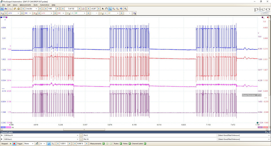
As you can see above, I’ve zoomed in on three messages. CAN H is on Channel A, CAN L is on Channel B and underneath we have one result of adding CAN H to CAN L and also one where CAN L has been subtracted from CAN H. You will notice that there is some interference on the CAN lines. It is picked up quite clearly in packet 1 on the A+B channel but when we subtract them the way the CAN controller does, any interference that was there no longer exists proving the CAN’s fault tolerance. Something else I've noticed, having looked at a few HGV and off-highway vehicles, is that the networks allow for a lot more interference. Normally with cars, when we add CAN H to CAN L, we end up with a very straight line at 5 V (2.5 V + 2.5 V = 5 and 3.5 V + 1.5 V = 5 V.) With trucks there always seems to be an allowable deviation of the 5 V. It’s never a huge amount but can be up to 0.4 V. However, when we look at the physical layer, A-B, everything is very even and allows us to use the inbuilt serial decode tool. A question we often get asked is what the spikes at the end of each byte are and is this something to be concerned about? The spikes, or ringing, can be down to a number of factors, but they are most often down to a limitation of the test leads. In order to eliminate these, it is advisable to use the 60 MHz scope probe, which will give a much cleaner signal. Please take a look at this forum post which describes the differences between the two leads in further detail. However, providing we know the limitations and are happy that what we are seeing is acceptable, then we can continue with the testing.
After running the truck back up to temperature, we start to experience the fault, with a slight hesitation, before the engine suddenly stops. Just as the customer had described. By leaving the scope to continue capturing after the event, meant we had both pre- and post data to look at.
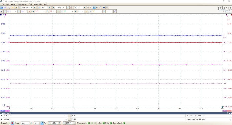
What we saw was complete network silence for two buffers, which totalled at 40 ms, before a single packet could be seen along with further silence. What we noticed, is that there were significantly less CAN traffic on the network. What now?
Well, wouldn’t it be good if we could identify what the packets of data actually meant or if we could tell which ECUs are online and not? Steve Smith has more resources in this forum topic, where he uses a number of techniques to help with decrypting the network to work out which ECU is which. There is a lot of information in this post, but what if we could make this even easier. With trucks and off-highway machines, the task of identifying ECUs is made simpler as they often use J1939 protocol. This is much more standardised than a typical car network, but it is still not that easy and manufacturers will throw their own spin on some controllers.
To begin with, we needed to perform a serial decode on the physical layer to start identifying individual IDs. To do this click Tools > Serial Decode. You will now have the opportunity to create a decoder by clicking Create and select CAN from the list. The setup box will appear, and you will be asked to select what data you will be decoding. In our case, we will be using A-B, which will be present in the dropdown box. This will only display channels that are active on the grid, so if any have been hidden from view you will not be able to select them. The next option is to select your threshold. This is the voltage you are telling the software to use as a ‘crossing point' for the decoder. A question was raised during our Q&A session, asking about CAN voltage thresholds for ECU fault detection. The honest answer is we do not know but we are actively working to find an answer. Please keep an eye on the forum for future updates and research into CAN. For the purpose of the test, we applied a crossing point of 1 V. Hysteresis can come right down to 20 mV, as we should be seeing a straight line up and down on our Math channel. You can find a great explanation of hysteresis and the effects on crossing points on page 157 of our User’s Guide. The Baud rate can sometimes be a mystery but there is a very simple way of determining what it is by using the time rulers in PicoScope. Using the marquee zoom, draw around a packet of data. Then you can use the time rulers to mark either side of the smallest bit. In the lower right-hand corner, you will see a figure in kHz. This will equate to your Baud rate.
With the settings done, our CAN decode setup should look something like this:

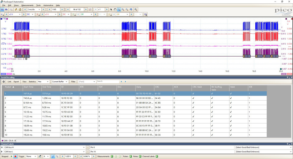
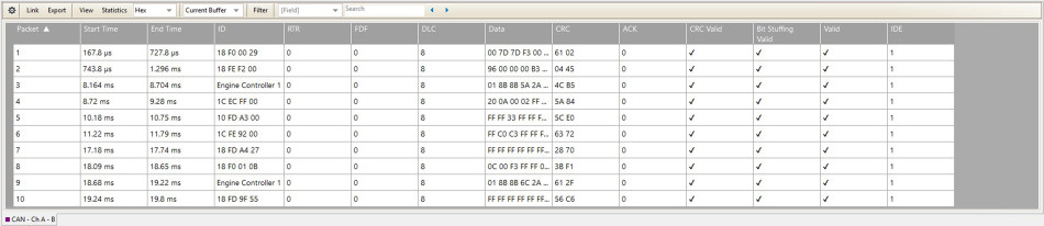
We will now be presented with a table where the packets of data have been converted into HEX code for the current buffer. I purposely selected the buffer just before the first ‘silent’ buffer (with no CAN traffic) as the one to start from as that is where the fault was not present. I have 10 packets of data that all decode correctly with no errors.
I mentioned earlier that J1939 is much more standardised than J2534. This means we can actually pull this data apart and start identifying IDs. By creating a link file we can convert the IDs into real words. From our serial data, we had a number of ECUs reporting a problem with the Engine ECM so it would make sense to look for the Engine ECM ID in our decode table. The first thing we needed to do was to determine which ID is the Engine ECM.
I won’t go into too much detail here, but I do want to show the possibilities that PicoScope can bring when it comes to serial decoding. We must remember, though, that PicoScope is not a dedicated CAN decoder/logger but an oscilloscope with limited decoder/logger features. That being said, there is still an awful lot we can do. To begin with, we need to understand how the message ID of a J1939 message is made up. The message header is made up of 29 Bits but to keep things simple we will look at the message in HEX. Each message has a unique Parameter Group Number, PGN, which contains the Suspect Parameter Number, SPN. All we are interested in this stage is the PGN as this points to a group table that refers to an ECU. To find the PGN in the header we look to the two middle bytes in an ID, for example – 0C F0 04 00 which means we are only interested in F0 04. We now convert F004 into a decimal, and by using a programmer calculator we get the number 61444. A quick search through the SAE standards for PGN 61444 confirms to us that this is for the Electronic Engine Controller 1. Therefore we can be confident that 0C F0 04 00 represented the Engine ECU or EEC1.
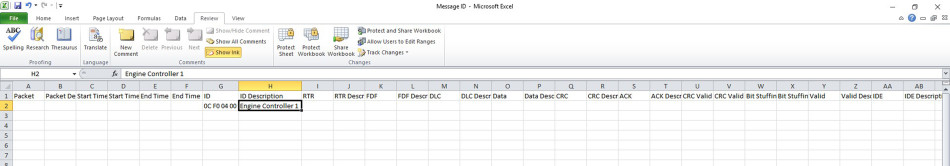
To then apply this to our decode table we need to fill in this information in our link file and save the file. To get this file click on the tab in the decode table marked Link. You will then see an option to Create File. Once clicked, it will ask you to save a CSV file. Select an appropriate location and then locate and open the saved CSV file. With the file open, there are a number of fields available that look like the decode table in PicoScope but with the additional ID Description header. Copy the ID from PicoScope exactly as it is in the decode table and add the description in the ID description column. For us, this was Engine Controller 1. Make sure you save any changes.
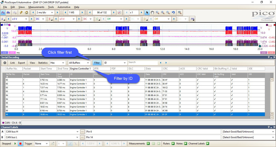
To tell PicoScope to look at this link file and replace any IDs with the description we have listed in the link file, click Link > Open, navigate to the link file location and select it. Once selected you should now see the IDs replaced with a language we can understand.
As luck would have it, it was the engine ECU we were looking for. Now we could sort through the data and look for this ID and any faults associated with it. We expanded the decoder to every buffer by selecting All Buffers in the dropdown box where the current buffer was selected. We could now export all this data to Excel for further analysis, or we could use the filter option in the decode table. Select Filter and then type the ID you would like to display, for us it was Engine Controller 1.
We knew the fault occurred at buffer 96, so started the search from there. We noticed that Engine Controller 1 was no longer present after buffer 96, and appeared to have gone offline despite this ID being very active throughout every buffer previous in the capture. Could this mean that the Engine ECU was at fault? It would make sense and we certainly had proof with our raw CAN Data. We could see that after buffer 96 something happened, the network was silenced, and from here on out the engine ECU was no longer online. This gave us enough reason to send the ECU away for testing, and sure enough, it was confirmed as faulty. A new Engine ECU was fitted, coded and reprogrammed and the vehicle was back on road.
This was an intriguing case and one that could have been costly for both the owner and us with the wrong diagnosis, but thanks to the PicoScope we had enough evidence to justify the path we took with the repair. As mentioned before, PicoScope is not a dedicated CAN decoder/logger. It is an oscilloscope with limited decoder/logger features, but we can discover much more by using the advanced features of the software. Hopefully, you can see that the possibilities are only limited by your imagination – oh, and time, of course!
Bart Kochowicz
November 05 2019
Very interesting, good insight into the case. I appreciate detailed description . One might expect better graphics, as it was mentioned before.
Niall Seddon
April 29 2019
are these images available in higher resolution as it is very difficult to see detail or as PICO data files